An inference-engineering primer
Quantization, explained from scratch: how AI models get smaller without getting dumber.
·20 min read
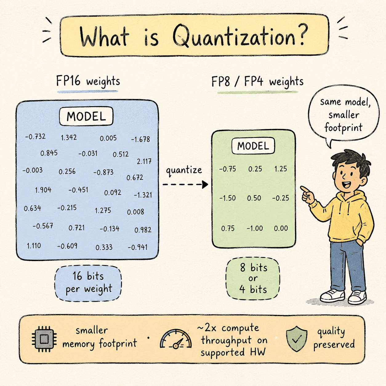
Large language models are made of weights — billions of numbers that the model learned during training. By default, each weight is stored as a 16-bit floating-point number (FP16 or BF16). For a 70B-parameter model, that's 140 GB of GPU memory just to hold the weights still.
Quantization is the process of converting those weights — and sometimes the activations and KV cache too — into a smaller numeric format. 8 bits instead of 16. Or 4. Or, on the latest hardware, microscaled 4-bit blocks.
Done well, quantization gives you:
- Lower memory footprint — fit the same model in less VRAM, or fit a bigger model in the VRAM you have.
- Higher throughput — more tokens per second on the same hardware.
- Lower latency — both TTFT (time to first token) and TPS (tokens per second) improve.
Done badly, quantization quietly degrades model quality. Subtle errors compound across every transformer layer and every generated token, and the model becomes a worse version of itself without any single output looking obviously broken.
This article covers the full picture: what quantization is, why it works, which formats you should use in 2026, the five major techniques and when to choose each, and how to actually do it in code on production-grade hardware (H100, B200). Where a free tier exists for learning, I'll point you at it.
1 · why it worksWhy quantization works.#
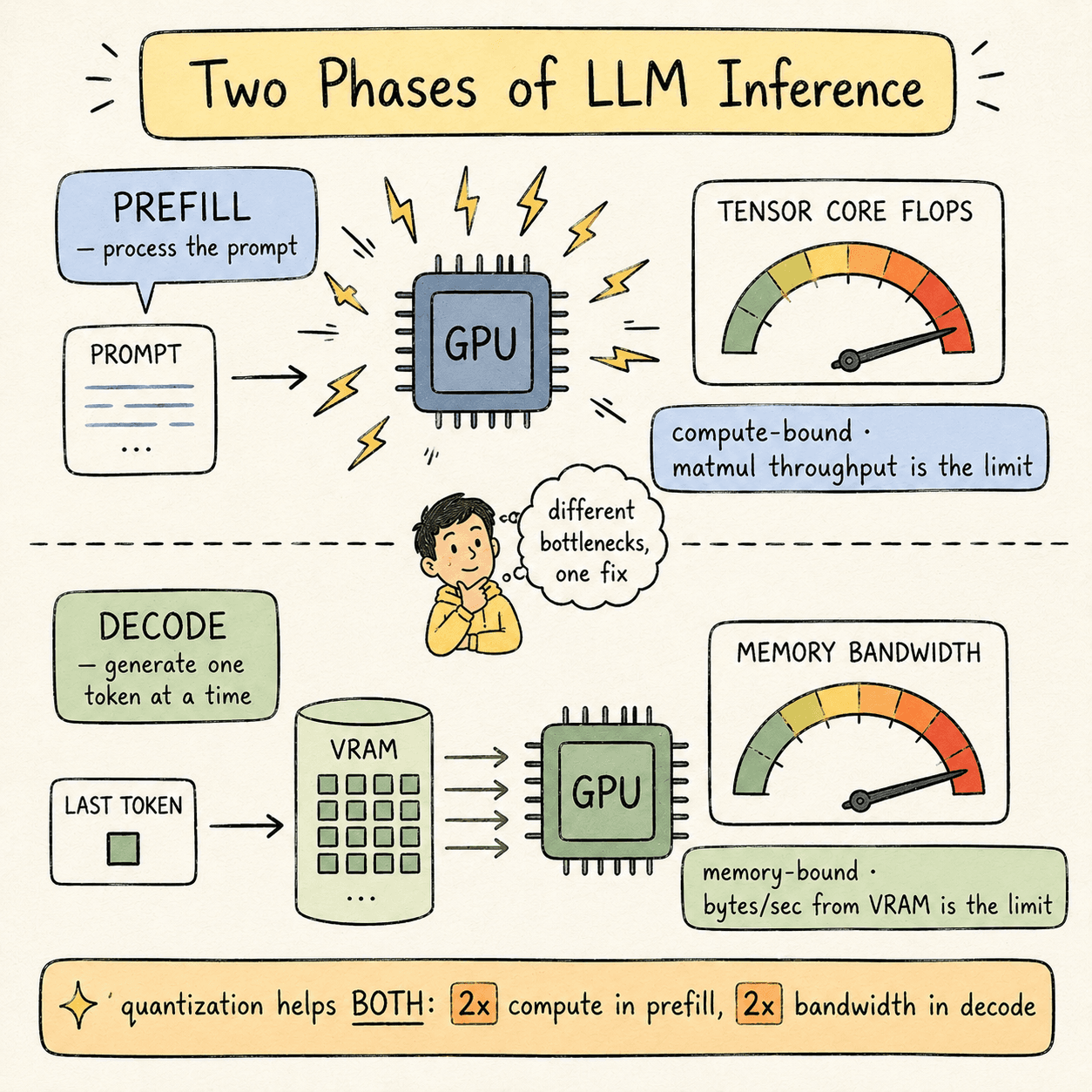
A language model serving request goes through two distinct phases:
Prefill phase. The model reads your prompt and computes the initial KV cache. This phase is compute-bound— the bottleneck is how fast the GPU's Tensor Cores can do matrix multiplications.
Decode phase. The model generates output tokens, one at a time. Each new token requires reading every model weight and the entire KV cache from GPU memory. This phase is memory-bound — the bottleneck is GPU memory bandwidth, not compute.
Quantization improves both phases, but for different reasons:
- In prefill, lower-precision matmul instructions execute at 2× the FLOPS on Tensor Cores. FP8 GEMM on Hopper runs at roughly twice the throughput of FP16 GEMM.
- In decode, each weight takes half as many bytes to load from VRAM, so effective memory bandwidth doubles.
In practice you don't get a clean 2× speedup. Dequantization overhead, kernel launch costs, and bookkeeping eat into the gain. A reasonable expectation: 30–50% better performance per precision drop (FP16 → FP8, FP8 → FP4) on hardware that natively supports the lower precision.
The “natively supports” caveat matters more than it sounds. We'll come back to it.
2 · number formatsNumber formats you need to know.#
Every numeric format has three properties that matter:
- Precision — number of bits used per value.
- Type — integer (no decimal) or floating-point (has a decimal).
- Scale factor — the multiplier that maps a low-precision value back to a higher-precision representation during inference.
These three properties determine two derived qualities:
- Dynamic range — the spread between the smallest and largest representable values.
- Granularity — how many parameters share a single scale factor.
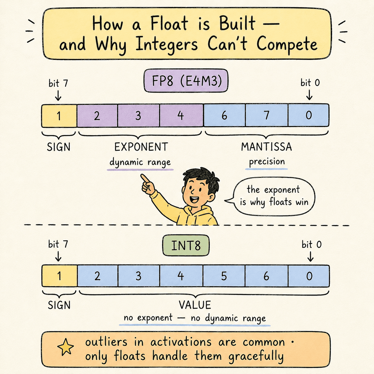
A floating-point number has three structural parts:
- Sign bit (1 bit) — positive or negative.
- Exponent (multiple bits) — magnitude.
- Mantissa (remaining bits) — significant digits.
Notation example: E4M3means 4 exponent bits + 3 mantissa bits + 1 sign bit = 8 bits total. That's one common variant of FP8.
Integer formats have only sign + value bits. No exponent means no dynamic range. This is why integers struggle to represent the outlier values that appear in real model activations. Floating-point formats handle outliers gracefully; integer formats crush them.
The formats currently used in production inference:
| Format | Bits | First seen on | Notes |
|---|---|---|---|
| FP16 | 16 | Pascal (2016) | Original inference baseline |
| BF16 | 16 | Ampere (2020) | Wider exponent than FP16 |
| FP8 | 8 | Hopper (2022) | Production sweet spot |
| MXFP8 | 8 | Blackwell (2024) | Microscaled FP8 — scale per 32 vals |
| FP4 | 4 | Blackwell (2024) | Aggressive — high quality risk |
| MXFP4 | 4 | Blackwell (2024) | Microscaled FP4 |
| NVFP4 | 4 | Blackwell (2024) | NVIDIA's 4-bit with 16-val blocks + global scale |
| NF4 | 4 | Software-defined | QLoRA's NormalFloat-4 |
| INT8 / INT4 | 8/4 | Various | Avoid for quality-sensitive workloads |
Rule of thumb:in datacenter production, prefer floating-point formats. Integers are fine for edge inference where techniques like GGUF's dynamic mixed-precision can compensate, but the lack of dynamic range makes them risky at scale.
3 · granularityGranularity.#
How many scale factors do you compute, and at what level?
- Tensor-level — one scale factor for the entire weight matrix. Cheap, imprecise, loses outliers.
- Channel-level — one scale factor per column (per output feature). Much better quality.
- Block-level — one scale factor per block of N values within each column. Best quality, more storage and compute overhead.
The Blackwell-generation formats — MXFP8, MXFP4, NVFP4 — are called microscaling formats. They compute a scale factor every 32 values (MXFP8/MXFP4) or every 16 values (NVFP4), with NVFP4 additionally using a 32-bit global scale factor on top. This is the cutting edge in 2026.
The microscaling tradeoff: each per-block scale factor takes up memory, but the quality gain (especially at 4 bits) is large enough to justify it. On Blackwell, Tensor Cores natively apply scale factors during the GEMM operation, so the runtime overhead is minimal.
4 · the sensitivity hierarchyThe sensitivity hierarchy.#
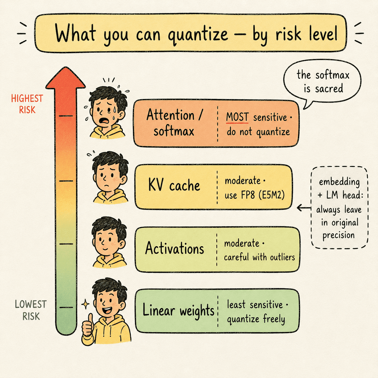
Not every component of a model handles quantization equally well. From least to most sensitive:
- Linear layer weights — least sensitive. Quantize freely.
- Activations — moderately sensitive. Quantize carefully.
- KV cache — moderately sensitive. Use high-dynamic-range formats.
- Attention internals — most sensitive. Softmax is almost never quantized.
Two refinements you should know:
- Early and late layers (input embedding, LM head) are usually left in original precision. Quantizing these tends to destroy output quality.
- Attention values compound errors across the sequence. Each attention step depends on all previous attention steps. A small quantization error at token 100 affects every attention computation through token 32,000. Softmax is especially fragile because it exponentiates its inputs.
A safe, defensible production recipe quantizes weights aggressively, activations carefully, the KV cache with a high-dynamic-range format, and leaves attention softmax alone.
5 · PTQ vs QATPost-training quantization vs quantization-aware training.#
There are two timing options for when quantization happens:
- Post-training quantization (PTQ) — take a finished FP16/BF16 model and convert its weights to a lower precision. Uses a calibration dataset (a small batch of representative inputs) to compute scale factors that preserve quality.
- Quantization-aware training (QAT) — train the model with quantization in the loop, so the final converged weights are already accurate at the target low precision. More expensive, but produces the highest-quality quantized models.
Examples of QAT releases: GPT-OSS in MXFP4, Kimi K2 Thinking in INT4.
If you're working with open-weight models from Hugging Face, you're almost always doing PTQ — you don't control training.
The leading PTQ tool today is NVIDIA TensorRT Model Optimizer (ModelOpt). Open source, supports pruning, distillation, sparsity, and quantization. Outputs are compatible with vLLM, SGLang, and TensorRT-LLM.
6 · the five techniquesThe five techniques (concept + code).#
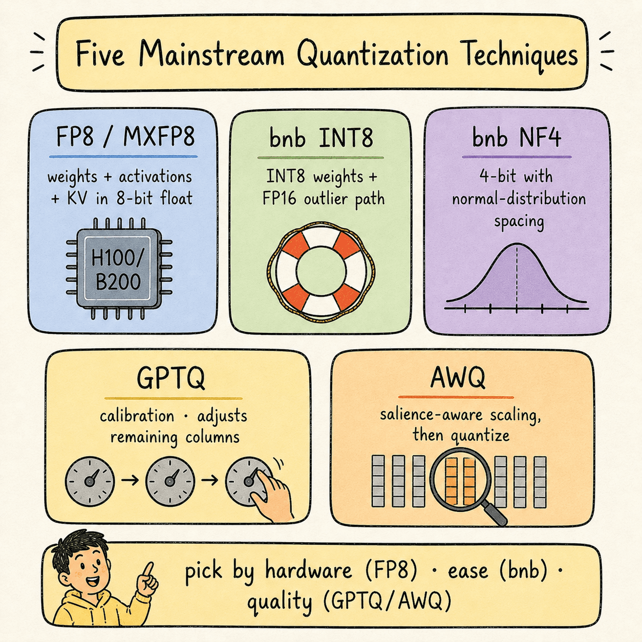
Five mainstream quantization techniques cover ~95% of real-world deployments.
6.1 — FP8 / MXFP8 (the production sweet spot on Hopper and newer)
What it is: quantize weights, activations, and KV cache to 8-bit floating point. On Hopper, FP8 GEMM runs at 2× the throughput of FP16. On Blackwell, MXFP8 with 32-value microscaling does the same but with better quality preservation.
Why it works: FP8 retains an exponent (E4M3 or E5M2), so it has enough dynamic range to preserve outliers. Hardware support means you get both the memory savings and the compute speedup at the same time.
Hardware required: L4 / L40S / H100 / H200 / B200 (Ada Lovelace or newer).
Free-tier alternative:none on T4 — FP8 needs Ada Lovelace at minimum. For learning the workflow without FP8, use INT8 or NF4 on a T4 Colab and mentally substitute “FP8 on H100” everywhere.
Code — FP8 PTQ with NVIDIA ModelOpt on H100:
import torch
import modelopt.torch.quantization as mtq
from transformers import AutoModelForCausalLM, AutoTokenizer

MODEL_ID = "meta-llama/Llama-3-70B-Instruct"

model = AutoModelForCausalLM.from_pretrained(
    MODEL_ID,
    torch_dtype=torch.bfloat16,
    device_map="cuda",
)
tokenizer = AutoTokenizer.from_pretrained(MODEL_ID)

# Calibration data — a small batch of representative prompts
def calib_loop():
    calib_texts = load_calibration_prompts(n=128)  # your eval distribution
    for text in calib_texts:
        inputs = tokenizer(text, return_tensors="pt", truncation=True,
                           max_length=2048).to(model.device)
        model(**inputs)

# Apply FP8 quantization config (weights + activations + KV cache)
config = mtq.FP8_DEFAULT_CFG
mtq.quantize(model, config, forward_loop=calib_loop)

# Export to TensorRT-LLM format for production serving
mtq.export(model, "./llama3-70b-fp8-export/")
Code — serving the FP8 model with vLLM:
from vllm import LLM, SamplingParams

llm = LLM(
    model="./llama3-70b-fp8-export/",
    quantization="fp8",
    kv_cache_dtype="fp8",        # FP8 KV cache too
    tensor_parallel_size=8,       # 8 H100s
)

prompts = ["Explain quantization in two sentences."]
outputs = llm.generate(prompts, SamplingParams(temperature=0, max_tokens=128))
print(outputs[0].outputs[0].text)
6.2 — bitsandbytes INT8 (LLM.int8())
What it is: weights are quantized to INT8, except for a small fraction (~1%) of outlier feature channels that stay in FP16. The two paths are merged after matmul.
Why it works: integers lack dynamic range, so naive INT8 destroys quality. bnb-INT8 detects outlier channels at runtime and routes them through a separate FP16 path, preserving the precision where it matters most.
Hardware required: runs on any GPU. But it only delivers speed improvementson Ampere or newer (A100+). On Turing (T4), it's a memory-only optimization that costs you speed.
Free-tier note:bnb-INT8 works on T4 Colab — that's where you can learn the mechanics. Just expect the model to run slower than FP16 on T4 because Turing lacks native INT8 Tensor Core support that bnb uses.
Code — bnb-INT8 on H100 (or A100):
import torch
from transformers import AutoModelForCausalLM, AutoTokenizer, BitsAndBytesConfig

MODEL_ID = "meta-llama/Llama-3-70B-Instruct"

bnb_config = BitsAndBytesConfig(
    load_in_8bit=True,
    llm_int8_threshold=6.0,           # outlier detection threshold
    llm_int8_has_fp16_weight=False,
)

model = AutoModelForCausalLM.from_pretrained(
    MODEL_ID,
    quantization_config=bnb_config,
    device_map="auto",
    low_cpu_mem_usage=True,
)
tokenizer = AutoTokenizer.from_pretrained(MODEL_ID)
6.3 — bitsandbytes NF4 (NormalFloat 4)
What it is: weights are quantized to a custom 4-bit format whose 16 representable values are spaced to be information-theoretically optimal for normal-distributed data — denser near zero, sparser at the extremes.
Why it works:trained neural network weights follow a roughly zero-centered normal distribution. A uniform INT4 grid wastes most of its budget on the tails. NF4's non-uniform grid places its 16 values where the weights actually are.
Hardware required: any GPU with CUDA. NF4 inference math is done in FP16, so the same Turing-era caveat applies — on T4 you get memory savings but minimal speed gain.
Free-tier note:NF4 on T4 Colab works well — best 4-bit option for the free tier. On H100 you'd typically reach for FP4/NVFP4 instead, but NF4 remains useful for QLoRA fine-tuning workflows.
Code — NF4 with double quantization:
import torch
from transformers import AutoModelForCausalLM, BitsAndBytesConfig

bnb_nf4_config = BitsAndBytesConfig(
    load_in_4bit=True,
    bnb_4bit_quant_type="nf4",          # NormalFloat 4
    bnb_4bit_compute_dtype=torch.bfloat16,
    bnb_4bit_use_double_quant=True,     # quantize the scale factors too
)

model = AutoModelForCausalLM.from_pretrained(
    "meta-llama/Llama-3-70B-Instruct",
    quantization_config=bnb_nf4_config,
    device_map="auto",
    low_cpu_mem_usage=True,
)
6.4 — GPTQ (calibration-based, activation-aware)
What it is: weights are quantized one column at a time. After each column is rounded, the remaining un-quantized columns are adjusted to compensate for the rounding error introduced. The adjustment is computed using the inverse Hessianof the layer's input — a matrix that captures which weight directions most affect the layer's output.
Why it works: naive quantization minimizes weight drift (||W - quantize(W)||). GPTQ minimizes output drift (||W·x - quantize(W)·x||) for representative inputs x. The output is what the next layer sees, so minimizing output drift is what preserves quality.
Hardware required: calibration runs on any GPU. Inference uses specialized INT4 kernels (ExLlamaV2, Marlin) that run well on Ampere and newer.
Free-tier note: on T4 Colab, auto-gptq install is currently broken due to wheel versioning issues. Use the pre-quantized GPTQ models published by model authors (e.g., Qwen/Qwen2.5-7B-Instruct-GPTQ-Int4) and load them via transformers' native loader.
Code — running GPTQ calibration yourself on H100:
from auto_gptq import AutoGPTQForCausalLM, BaseQuantizeConfig
from transformers import AutoTokenizer
from datasets import load_dataset
import random

MODEL_ID = "meta-llama/Llama-3-70B-Instruct"
N_CALIB = 128
CALIB_SEQ_LEN = 2048

tokenizer = AutoTokenizer.from_pretrained(MODEL_ID)

# Build calibration set — must be representative of deployment traffic
raw = load_dataset("wikitext", "wikitext-2-raw-v1", split="train")
texts = random.sample([t for t in raw["text"] if len(t) > 500], N_CALIB)
calib = [
    {"input_ids": tokenizer(t, return_tensors="pt", truncation=True,
                            max_length=CALIB_SEQ_LEN).input_ids,
     "attention_mask": tokenizer(t, return_tensors="pt", truncation=True,
                                 max_length=CALIB_SEQ_LEN).attention_mask}
    for t in texts
]

quant_config = BaseQuantizeConfig(
    bits=4,
    group_size=128,        # block-level granularity
    desc_act=True,         # activation-magnitude column ordering (better quality)
    damp_percent=0.01,
    sym=True,
)

model = AutoGPTQForCausalLM.from_pretrained(MODEL_ID, quantize_config=quant_config)
model.quantize(calib)
model.save_quantized("./llama3-70b-gptq-int4/", use_safetensors=True)
Code — loading a pre-quantized GPTQ model for serving:
from transformers import AutoModelForCausalLM, AutoTokenizer

MODEL_ID = "Qwen/Qwen2.5-7B-Instruct-GPTQ-Int4"
tokenizer = AutoTokenizer.from_pretrained(MODEL_ID)
model = AutoModelForCausalLM.from_pretrained(
    MODEL_ID,
    device_map="auto",
    low_cpu_mem_usage=True,
)
6.5 — AWQ (Activation-aware Weight Quantization)
What it is: before quantization, AWQ identifies the salient weight columns — roughly the top 1% of columns that are multiplied by large-magnitude activation channels. Those columns are scaled upbefore quantization so they land on more precise values, and the corresponding activations are scaled down by the same factor (folded into the previous LayerNorm at compile time, so there's no runtime cost).
Why it works:not all weights contribute equally to the layer's output. The weights multiplied by high-magnitude activations dominate the output; the rest are background. Protecting the dominant ones at quantization time preserves output quality without slowing down inference.
Hardware required: AWQ kernels run well on Ampere and newer. AWQ typically beats GPTQ on inference speed because the kernel is simpler — no per-column scale logic at inference, just standard INT4 matmul plus a folded LayerNorm rescale.
Free-tier note: autoawq installs more reliably on T4 Colab than auto-gptq does. You can either calibrate locally or load a pre-quantized model like Qwen/Qwen2.5-7B-Instruct-AWQ.
Code — AWQ calibration and quantization on H100:
from awq import AutoAWQForCausalLM
from transformers import AutoTokenizer

MODEL_ID = "meta-llama/Llama-3-70B-Instruct"
QUANT_PATH = "./llama3-70b-awq-int4/"

tokenizer = AutoTokenizer.from_pretrained(MODEL_ID)
model = AutoAWQForCausalLM.from_pretrained(MODEL_ID, device_map="cuda")

quant_config = {
    "zero_point": True,
    "q_group_size": 128,
    "w_bit": 4,
    "version": "GEMM",     # GEMM is faster than GEMV on most modern GPUs
}

model.quantize(tokenizer, quant_config=quant_config)
model.save_quantized(QUANT_PATH)
tokenizer.save_pretrained(QUANT_PATH)
Code — serving an AWQ model with vLLM:
from vllm import LLM, SamplingParams

llm = LLM(
    model="./llama3-70b-awq-int4/",
    quantization="awq",
    tensor_parallel_size=2,    # 2 H100s for a 70B AWQ model
)
7 · kv cache quantizationKV cache quantization — the biggest VRAM lever.#
The KV cache stores the key and value vectors of every previously generated token, so the attention mechanism can attend back to them without recomputing.
KV cache size scales linearly with:
- Sequence length
- Number of transformer layers
- Number of attention heads (smaller with GQA/MQA)
- Head dimension
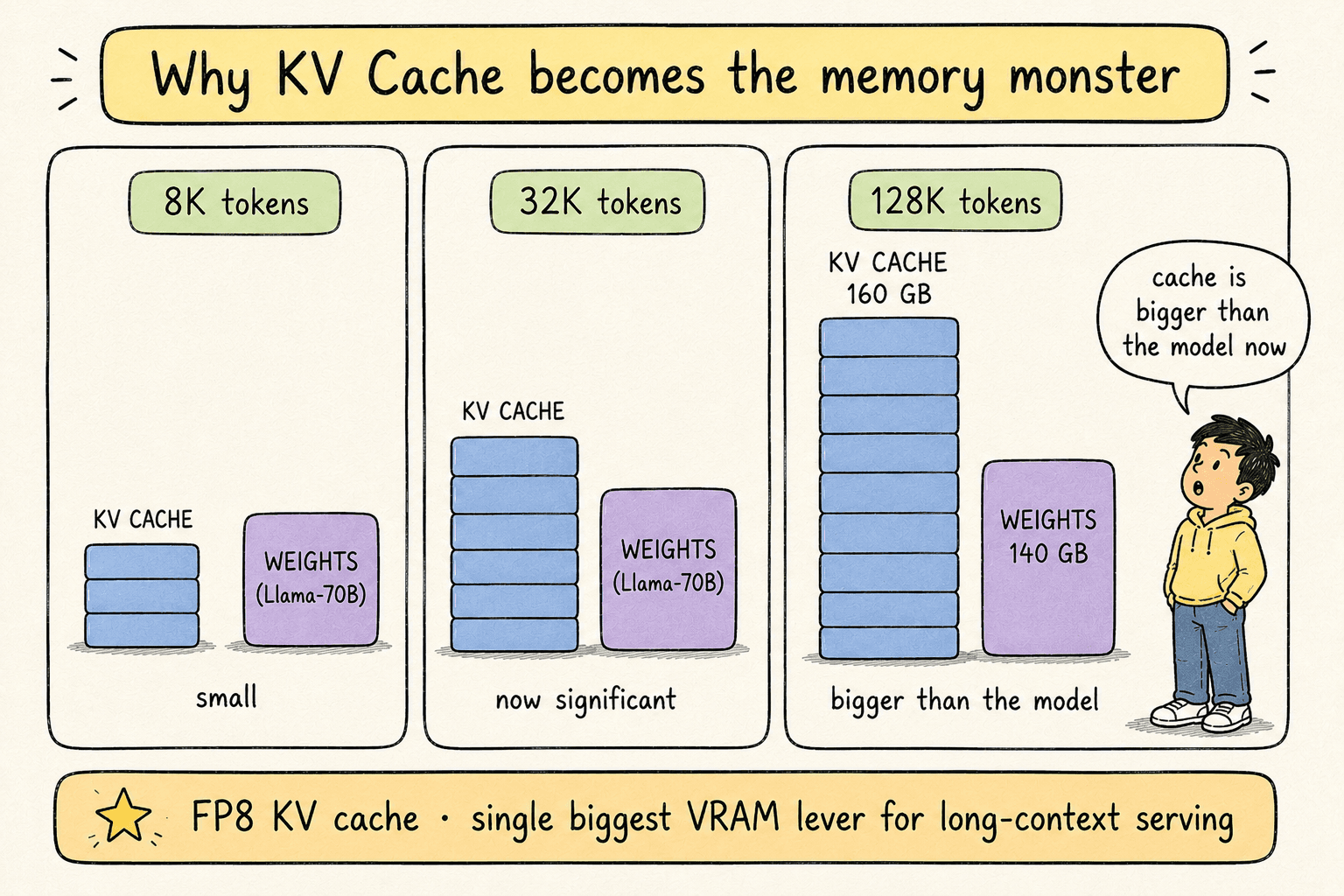
For short contexts the KV cache is invisible. For long contexts it becomes the dominant VRAM consumer:
| Model | Context length | Approx. KV cache size |
|---|---|---|
| Llama-3-8B | 8K tokens | ~4 GB |
| Llama-3-70B | 32K tokens | ~40 GB |
| Llama-3-70B | 128K tokens | ~160 GB |
For long-context serving, quantizing the KV cache from FP16 to FP8 is the single biggest VRAM lever you can pull.
Why it's risky:the KV cache for each token is consumed by every subsequent token. Errors in token 5's cached K/V propagate to every attention computation for tokens 6 through N. Compounded errors are real.
Safe choice: FP8 KV cache (E5M2 has higher dynamic range than E4M3 — prefer it for the cache). Quality cost is typically negligible.
Aggressive choice: INT8 KV cache. Cheaper but quality cost can be visible on long contexts.
Code — FP8 KV cache with vLLM on H100:
from vllm import LLM

llm = LLM(
    model="meta-llama/Llama-3-70B-Instruct",
    quantization="fp8",
    kv_cache_dtype="fp8_e5m2",       # E5M2 for higher dynamic range
    max_model_len=131072,             # 128K context
    tensor_parallel_size=4,
)
Free-tier note: for learning, the HQQlibrary supports KV cache quantization with transformers on any GPU. On T4 the savings exist but you won't see speed gains.
8 · weights-only vs weights+activationsWeights-only vs weights + activations.#
Every linear layer in a transformer computes:
output = (W × x) + bYou can quantize either side:
| Scheme | What's quantized | Matmul precision |
|---|---|---|
| W-only | weights only | FP16 / BF16 |
| W+A | weights and activations | low precision (INT8, FP8, FP4) |
Naming convention: W4A16 = weights INT4, activations FP16. W8A8 = both INT8. W4A8 = weights INT4, activations INT8.
bnb-INT8, bnb-NF4, GPTQ, AWQ — all of these are W-onlyby default. The weights are quantized; the actual matmul runs in FP16 after on-the-fly dequantization. You save memory but the matmul doesn't get faster.
Real speed gains come from quantizing both sides, which lets the matmul itself run at low precision on the Tensor Cores:
| Hardware | Native low-precision matmul |
|---|---|
| T4 (Turing) | none — quantization is memory-only |
| A100 (Ampere) | INT8, INT4 |
| H100 (Hopper) | INT8, INT4, FP8 |
| B200 (Blackwell) | INT8, INT4, FP8, MXFP8, MXFP4, NVFP4 |
This is why the book's production recommendation is FP8 W8A8 on H100 or MXFP8 on B200. Both halves of the matmul run at low precision; you get the memory savings and the compute speedup simultaneously.
Operationally: start with W-only on safe-to-quantize components (weights, KV cache). Add activation quantization once you have hardware that natively supports the corresponding low-precision matmul.
9 · measuring qualityMeasuring quality after quantization.#
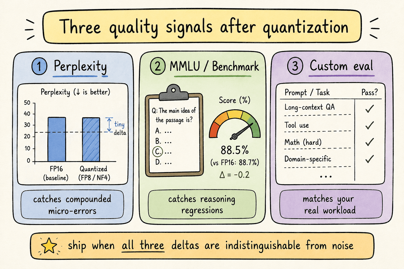
The standard for production-ready quantization is zero perceptible quality loss. You verify with three signals:
1. Perplexityon a held-out text corpus (typically WikiText-2). Perplexity measures how “surprised” the model is by real text. Lower is better. Perplexity catches subtle compounded errors that other metrics miss.
2. Benchmark accuracy on a public benchmark like MMLU or SWE-bench. Tests reasoning and knowledge.
3. Custom evaluation on prompts that match your real production traffic. This is the most honest signal — public benchmarks rarely match your workload distribution.
What you want: a difference indistinguishable from noise on all three. LLMs are non-deterministic, so scores vary slightly run-to-run.
Code — perplexity measurement on WikiText-2:
import torch
from datasets import load_dataset
from tqdm import tqdm

@torch.no_grad()
def perplexity(model, tokenizer, stride=512, max_length=2048, max_chunks=200):
    text = "\n\n".join(t for t in load_dataset(
        "wikitext", "wikitext-2-raw-v1", split="test")["text"] if t.strip())
    input_ids = tokenizer(text, return_tensors="pt").input_ids.to(model.device)
    nlls, prev_end, n = [], 0, 0
    for begin in tqdm(range(0, input_ids.size(1), stride)):
        end = min(begin + max_length, input_ids.size(1))
        trg_len = end - prev_end
        ids = input_ids[:, begin:end]
        targets = ids.clone()
        targets[:, :-trg_len] = -100
        outputs = model(ids, labels=targets)
        nlls.append(outputs.loss.float() * trg_len)
        prev_end = end
        n += 1
        if end == input_ids.size(1) or n >= max_chunks:
            break
    total = (n - 1) * stride + trg_len
    return torch.exp(torch.stack(nlls).sum() / total).item()
Code — MMLU evaluation via lm-eval-harness:
# Install: pip install lm-eval
# Run from CLI:

# lm_eval --model hf \
#   --model_args pretrained=meta-llama/Llama-3-70B-Instruct,dtype=fp8 \
#   --tasks mmlu \
#   --num_fewshot 5 \
#   --batch_size 8 \
#   --output_path ./eval_results/
Code — measuring TTFT and TPS:
import time
import torch

@torch.no_grad()
def measure_latency(model, tokenizer, prompt, max_new_tokens=128,
                    warmup=2, timed=5):
    inputs = tokenizer(prompt, return_tensors="pt").to(model.device)
    input_len = inputs.input_ids.shape[1]

    # Warmup — first runs include kernel compile and cache allocation
    for _ in range(warmup):
        _ = model.generate(**inputs, max_new_tokens=max_new_tokens,
                           do_sample=False)
    torch.cuda.synchronize()

    # TTFT: generate exactly 1 token
    ttft_times = []
    for _ in range(timed):
        torch.cuda.synchronize()
        t0 = time.perf_counter()
        _ = model.generate(**inputs, max_new_tokens=1, do_sample=False)
        torch.cuda.synchronize()
        ttft_times.append(time.perf_counter() - t0)

    # TPS: full generation
    full_times = []
    for _ in range(timed):
        torch.cuda.synchronize()
        t0 = time.perf_counter()
        out = model.generate(**inputs, max_new_tokens=max_new_tokens,
                             do_sample=False)
        torch.cuda.synchronize()
        full_times.append(time.perf_counter() - t0)

    avg_ttft = sum(ttft_times) / len(ttft_times)
    avg_total = sum(full_times) / len(full_times)
    generated = out.shape[1] - input_len
    return {
        "ttft_ms": avg_ttft * 1000,
        "tps": generated / avg_total,
    }
Note the two non-negotiables in that measurement code:
- Warmup runs — the first generation call includes CUDA kernel compilation, KV cache allocation, and GPU power-state ramp-up. Without warmup your numbers are 2–10× worse than reality.
torch.cuda.synchronize()— GPU work is asynchronous. Without syncing,time.perf_counter()measures when you queued the work, not when it finished. You'd report fictional speed.
10 · hardware tiersHardware tier reference.#
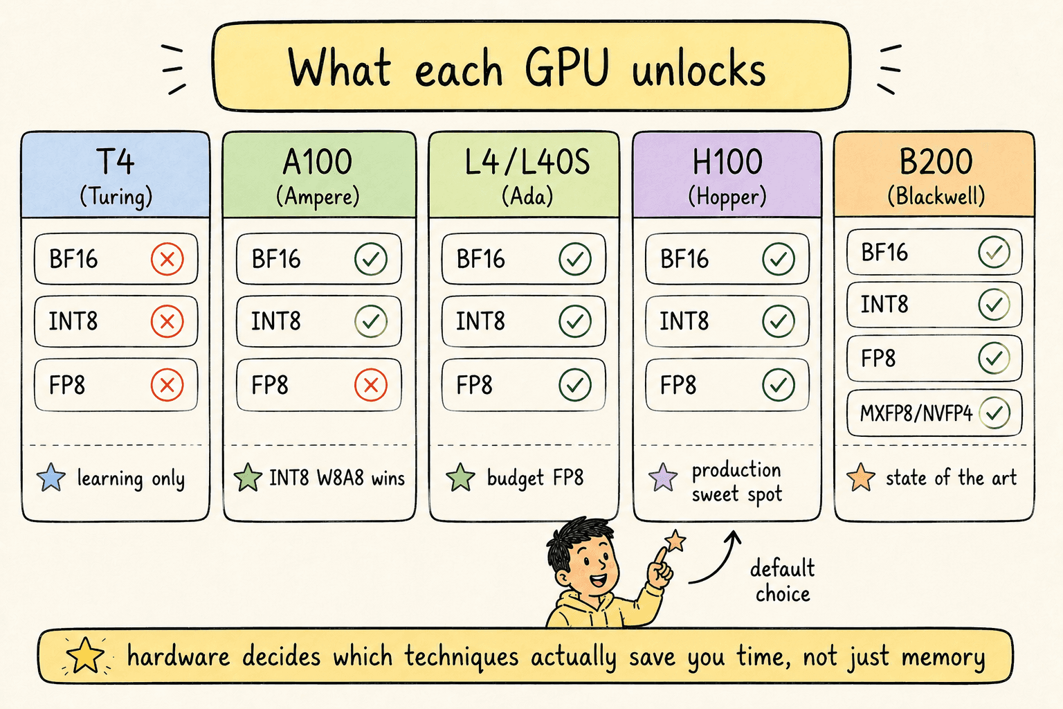
Every quantization decision is gated by what your hardware natively supports. The current landscape:
| GPU | Architecture | Year | BF16 | INT8 | FP8 | MXFP8 / NVFP4 |
|---|---|---|---|---|---|---|
| T4 | Turing | 2018 | ✗ | ✗* | ✗ | ✗ |
| A100 | Ampere | 2020 | ✓ | ✓ | ✗ | ✗ |
| L4 / L40S | Ada Lovelace | 2022 | ✓ | ✓ | ✓ | ✗ |
| H100 | Hopper | 2022 | ✓ | ✓ | ✓ | ✗ |
| B200 | Blackwell | 2024 | ✓ | ✓ | ✓ | ✓ |
*INT8 runs on T4 but lacks the Tensor Core path used by modern quantization libraries — effectively memory-only.
Practical decision tree:
- Deploying on B200? Use MXFP8 for weights+activations, MXFP8/NVFP4 KV cache. State of the art.
- Deploying on H100? Use FP8 W8A8 with FP8 KV cache. Production sweet spot.
- Deploying on A100? Use INT8 W8A8 or AWQ W4A16. Real speed wins.
- Deploying on L4 / L40S (budget)? FP8 works. Lower throughput than H100 but cheaper per request.
- Learning on T4 Colab? Use bnb-INT8 or NF4for the workflow. Accept memory-only wins. Move to L4+ when you're past learning.
11 · a safe production recipeA safe production recipe.#
If you only remember one full recipe, remember this one. It's a defensible starting point for almost any model on H100-class hardware.
| Component | Format | Rationale |
|---|---|---|
| Linear weights | FP8 (E4M3) | Quantize freely — least sensitive |
| Activations | FP8 (E4M3) | Dynamic per-token quantization |
| KV cache | FP8 (E5M2) | Higher dynamic range for cache |
| Attention softmax | FP16 / BF16 | Almost never quantize |
| Input embedding | FP16 / BF16 | Sensitive — leave alone |
| LM head | FP16 / BF16 | Sensitive — leave alone |
Then validate with: WikiText-2 perplexity, MMLU (5-shot), and your custom eval. Confirm the gap to baseline is statistical noise on all three. Ship.
12 · key takeawaysKey takeaways.#
- Quantization is two things at once. A memory optimization (always) and a compute optimization (only when hardware supports the low-precision matmul). On modern hardware you get both. On older hardware you get one.
- FP8 W8A8 on H100 is the production sweet spot in 2026. Half the memory, ~2× the compute throughput, near-zero quality loss. MXFP8 on B200 is the next step up.
- Floating point beats integer in production. The exponent bits give floats the dynamic range needed to preserve outliers. Use FP8, FP4, NF4 — avoid INT8 and INT4 for quality-sensitive workloads when you have a choice.
- The sensitivity hierarchy is non-negotiable. Weights → activations → KV cache → attention. Quantize aggressively at the bottom, never at the top.
- KV cache quantization is the biggest VRAM lever for long contexts. For 32K+ token serving, FP8 KV cache is mandatory.
- Quantization is a scale, not a switch.If quality is at risk, you have two dials: raise precision (FP4 → FP8) or shrink scope (W+A → W only). You don't have to pick between “fully quantized” and “FP16”.
- Always measure with three signals. Perplexity (catches compounded micro-errors), benchmark accuracy (catches reasoning regressions), custom eval (catches workload-specific issues). One signal is never enough.
- Pre-quantized models are the practical shortcut. For mainstream models — Llama, Qwen, Mistral, DeepSeek — official quantized releases exist on Hugging Face. Use them when you don't need a custom calibration distribution.